POSTED ON 05 DEC 2019
READING TIME: 11 MINUTES
An introduction to hypothesis testing


As part of the ongoing development of our VisiMetrix platform we are faced with the need to make decisions about how best to analyse massive datasets. We want to help users make decisions when looking at data. Sometimes though it’s too expensive to check all the data or it’s so complicated that it's easy to make an incorrect assumption and be led away in the wrong direction.
In cases like this, hypothesis testing can help by providing a degree of confidence that either our observations are real, or the changes we’ve made have, in fact, made a difference.
In cases where a complete examination of the underlying data set is impossible - perhaps all the data is not yet available or is simply too expensive to process all of it - we have found the following statistical tests to be very helpful.
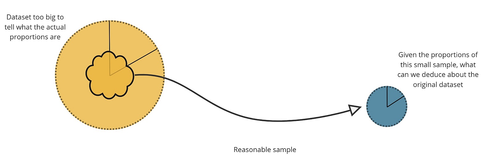
1-Sample Z-Test
VisiMetrix monitors large telecom networks, and in some cases its data will suggest that new software or hardware elements should be added to the network to improve overall performance. Since changing telecom networks is costly, we need to determine whether this change would be worthwhile by verifying that a sizeable proportion of the underlying traffic matches a well-defined profile. Unfortunately, checking such vast quantities of data is extremely compute and time-intensive.
In cases like this, a test known as the 1-sample Z-test can be applied to a sample of the data to determine if the network infrastructure change is, in fact, worthwhile implementing.
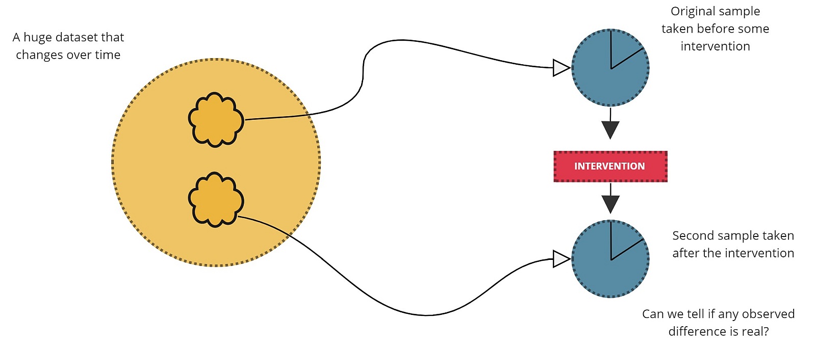
2-Sample Paired T-Test
When VisiMetrix draws the attention of a telco’s operations team to a history of PDP creation (user connectivity) errors, they will often apply a configuration change to their underlying network to correct this. However, since things like PDP creation errors are, for the most part, rare, it can be a challenge to validate that a configuration change has, in fact, corrected connection failures for real end-customers.
In cases like this, a 2-sample paired t-test can be applied to samples taken before and after the configuration changes to confirm that any reduction in errors was, in fact, real, and not just a random artifact of the data.
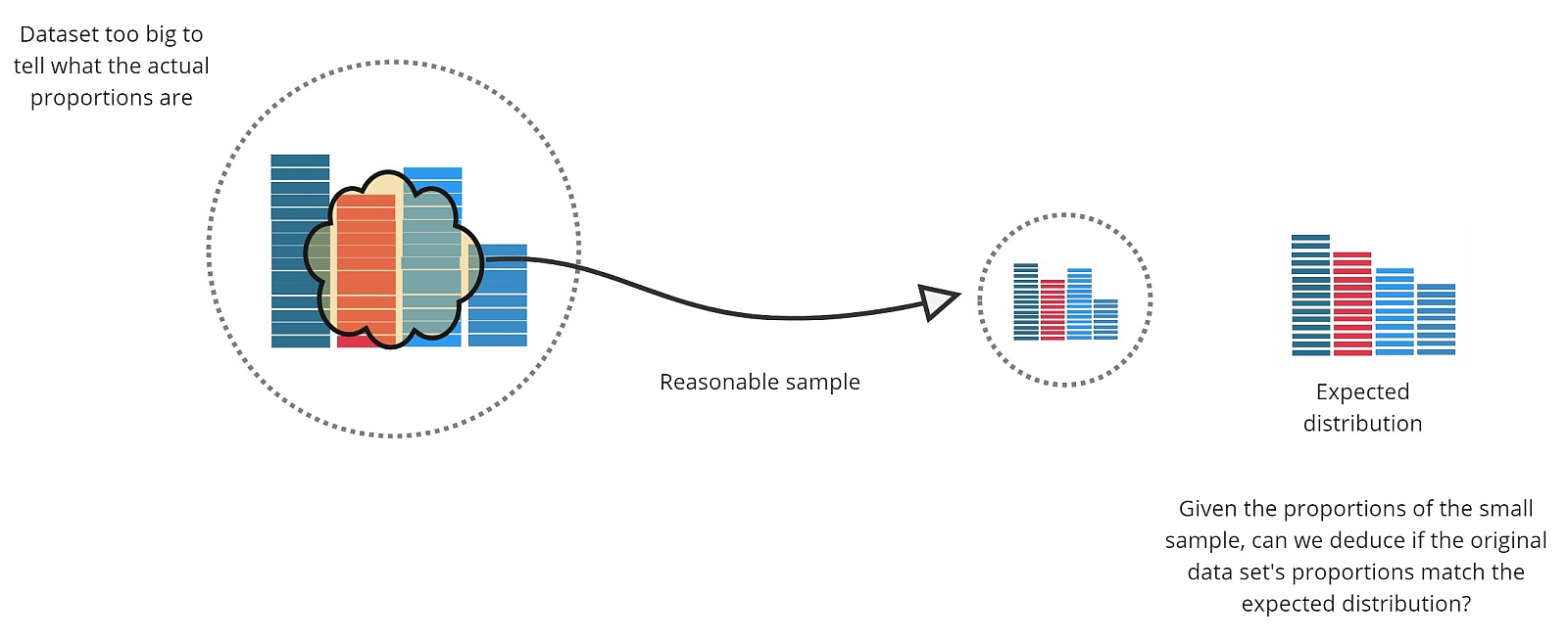
Chi-Square Goodness of Fit
When a telco is planning new hardware deployments, they can use information from their monitoring infrastructure to understand the pre-upgrade state of the network. Looking beyond that they have to make some assumptions about traffic patterns as far as 2-3 years in the future.
- Expected future event volumes
- Expected distribution for each event type
They will use these predicted volumes to dimension new hardware, network, and other infrastructure. Once deployed, it is critical to validate these sizing assumptions early on. The challenge, however, is that the traffic soon after an upgrade will be nowhere near the upper limit of what was sized so it would be difficult to tell whether or not the upgrades will be able to support the predicted traffic volumes in the coming years.
The challenge here is to validate the dimensioning assumptions in advance of peak traffic. Using the fact that the proportions of event types should not differ significantly pre and post upgrade we can apply a Chi-Square Goodness of Fit test to the initially limited production data and used to confirm that the observed distribution is as-expected.
Once we know this, we can be confident that the deployed hardware will support the eventual load. This test is performed regularly, to catch any changes in user behaviour over time that might affect the proportions.
The purpose of this series of blog posts is to provide an introduction to hypothesis testing, and the types of problems to which it can be applied. At the end of this post I will present a cheat sheet that will help you decide when to use which type of test. The following posts will go into more depth for each test, and provide a code sample for how to calculate it.
Hypothesis Testing
Hypothesis testing is a statistical method that can be used to make decisions about a data set without having to examine every element in that dataset. For example, imagine you have a software system that processes billions of events per hour. Events are grouped into transactions of, say, hundreds of events. Your product owner has identified a candidate product feature that could provide real customer value but only if at least 80% of the transactions over the last 12 months contain events that match a given set of criteria (profile).
Now we have a problem. It will take weeks to check to process 12 months of events.
Why are we bothering to take a sample? Because we want to make a decision, and checking every element in the set might be too difficult (billions of events), or just impossible (testing food means destroying it).
The issues then become:
- There is something we want to know about the entire population, but we can’t interrogate all of it.
- We sample the population and learn something about that sample, but since it’s only a sample, we can’t be sure that it is, in fact, representative of the entire population.
- Finally, what - if anything - can we guess about the population, given what we’ve learnt about the sample?
This can all get very heavy, very quickly, so I’ll give a quick example of what a hypothesis test does. In this example we have a data set that’s so large we can't process all of it to get an answer, so we have to sample it, and then check what conclusions we can deduce from this sample.
Example:
- Suppose your software application is processing billions of transactions per hour.
- Your product owner has asked you to implement some new way to process these transactions, but it’s only a worthwhile feature to implement if at least 80% of the transactions - over the whole of the last year - match a given profile.
- Now suppose that a check to see if a given transaction fits this profile was so expensive to calculate that it would take weeks to check all of them.
- So, instead, you sample just 1,000 transactions and find out that 82% of the sampled transactions have the required profile.
What can we say about all these billions of transactions, given what we have learnt about just this sample of 1,000? This is where the null hypothesis and alternative hypothesis come into play.
Null and Alternative Hypothesis
A hypothesis test starts with making two hypotheses
- The null hypothesis - in general, this is a “suppose there’s nothing to see here” case.
- The alternative hypothesis - this is what we’re checking for.
The test works by assuming the null hypothesis is true and then checking to see how likely a sample fits into that hypothesis. If it’s not likely enough, then we can suggest the alternative hypothesis is true.
Before taking the sample a significance level is selected. By convention this is 5% - but be advised, this is only a convention, and you must choose this with care. Later on, you will be making a judgement based on a derived probability by comparing it to this significance, so it’s important to consider the significance level before taking the sample.
Technically, this makes this kind of hypothesis test a significance test - we’re not proving anything. We are only deciding that, on the balance of probabilities, given how much risk we’re willing to take, that we’re happy to accept that something is likely enough to be true.
Does that sound vague? It should. There are reasons to be very careful about the kinds of assumptions you should be willing to make based on the results of these tests.
In short, these tests aren’t about certainty, they’re about confidence.
In our example, we would start by assuming this null hypothesis is true:
Exactly 80% of the transactions match the profile
Or in more formal language:
p(profile) **\=** 0.8
What we want to do now is imagine the following. Note, we don’t actually have to do the following, this is just here to explain to you why this all works.
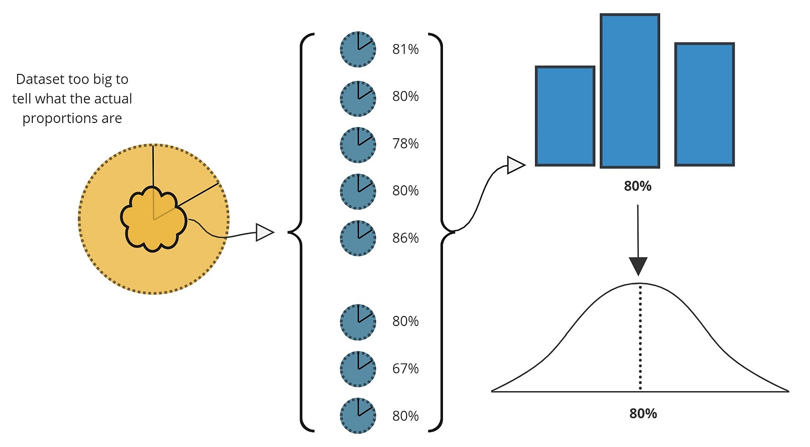
- Imagine what would happen if we were to take lots of samples from a population where the proportion was exactly 80%
- Each sample we took would have a different proportion; but we'd expect most of them to be near enough to the "real" one of 80%
- If we count how many of each proportion we get, the result is a histogram where the "real" proportion has the highest bar.
- Eventually, if we were to take more and more samples, this would tend towards a normal curve, centred around 80%
Now we have a curve - for a fictional population that matches our null hypothesis - with which we can compare our sample.
Sample and Compare to Null Hypothesis
So, how do we check our sample against this null hypothesis curve? First, we define our alternative hypothesis - i.e. this is the thing we’re trying to prove. For the kinds of tests we’re talking about here, this must be related to the null hypothesis - i.e. it must be comparing the same terms, just comparing them with a different operator.
In our example, because we have the null hypothesis:
Exactly 80% of the transactions match the profile
We would consider this as our alternative hypothesis:
More than 80% of the transactions match the profile
Or in more formal language:
p(profile) > 0.8
Finally, we compare our sample proportion (in our example this was 82%) to the curve for the null hypothesis, and we figure out how likely it is that this sample could have come from a population where the proportion was, in fact, exactly 80%.
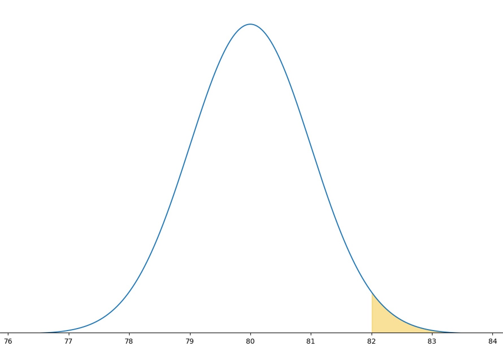
In our example, since we’re checking how likely it is that our real population proportion is greater than 80% (our assumed null hypothesis population proportion), we are, in effect, comparing:
- The area under this curve to the right of where our sample result is.
- To the total area under this curve.
This fraction is the probability of how likely it is that our sample came from a population that had a proportion that matched our null hypothesis.
Drawing conclusions about the sample
All of the tests that follow derive a result called a p-value. These values are often misunderstood. This misunderstanding can lead the tester to make certain assumptions about the underlying population that cannot be justified.
The p-value is the probability that the sample result could have occurred if the null hypothesis were true.
So, a p-value has no meaning outside of the given sample, and cannot be related to any other sample or p-value, and doesn't give an indication of how accurate the sample value is. So, in our example, had we calculated a p-value of 4%, the following significance levels would have caused us to draw the following conclusions:
| Significance | Conclusions |
|---|---|
| 5% |
- The p-value of 4% is less than the significance of 5%.
- So, the probability of this sample coming from a population with the values assumed by the null hypothesis is not significant.
- So, we can reject the null hypothesis, which suggests the alternative hypothesis. NOTE: this doesn’t prove the alternative hypothesis; only that we can feel a degree of confidence that more than 80% of the transactions match our profile.
- We cannot say anything else about the actual value of the proportion of the underlying population - i.e. we can’t say that it’s likely to be 82%, or even close to 82%
| | 1% |
- The p-value of 4% is greater than (or equal to) the significance of 1%.
- So, the probability of this sample coming from a population with the values assumed by the null hypothesis is significant.
- We cannot reject the null hypothesis, i.e. we can’t feel confident that the sample came from a population different from the one assumed by the null hypothesis.
- We cannot say anything else about the actual value of the proportion of the underlying population - i.e. we can’t say that it’s likely to be less than 80%
|
What Next?
This above example is for a test comparing proportions, but a different test would be required depending on what it was that you were comparing. This figure below offers a guide as to which test to apply depending on the nature of the data, and the observations you’re looking to make.
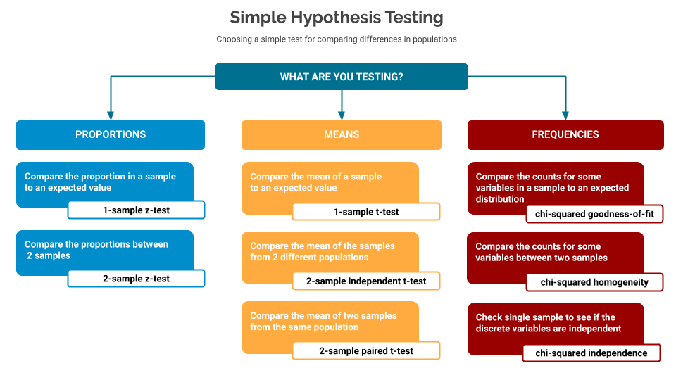
The rest of this series of blog posts will explain - with examples - when each of these different test types is applicable, and will include sample code for each of them.