Predicting RAN congestion with LSTM

There is no doubt that the pandemic has changed the way we live and work. The patterns of our working day have shifted, as has our use of technology to support these changes. According to an OECD study, “demand for broadband communication services has soared, with some operators experiencing as much as a 60% increase in internet traffic compared to before the crisis”.

In addition, telecom operators have noticed an increasing demand for high-speed data applications (e.g., high-quality video streaming, online games, video calls) that have a massive impact on their networks. In their Visual Networking Index, Cisco projects that video will account for 77% of total mobile data traffic by 2022, representing a six-fold increase since 2017, ​growing at a Compound Annual Growth Rate (CAGR) of 46% over the period 2017-2022.

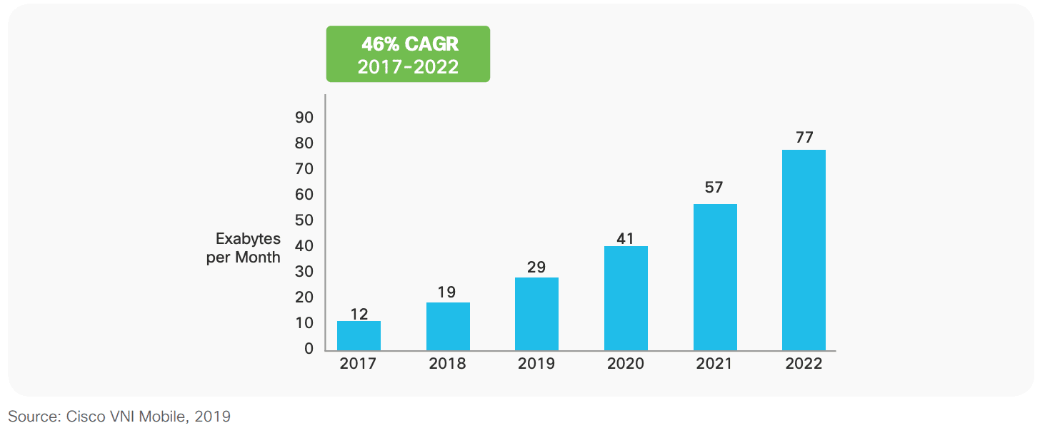Figure 1. Cisco forecasts 46% CAGR in mobile data traffic

These changes create a set of unique problems for the network operators. Already stretched networks must adjust to increasing bandwidth demands while continuing to meet the quality of service standards. Network operators must continually monitor and optimise their network while simultaneously forecasting future usage to aid capacity infrastructure investment. Striking this balance will ensure customers remain connected, happy and valued.

One of the biggest challenges when trying to predict Radio Access Network (RAN) congestion in mobile networks is the sheer number of cells. There are thousands of cells in the network and each behaves differently based on characteristics such as physical location and population density. Compounding this problem are seasonal patterns over days, weeks, and months.

As part of our ongoing development of our VisiMetrix, we wanted to determine if we could help users by predicting RAN congestion. Could we effectively predict RAN congestion up to 7 days into the future and, thus, provide an early warning system for network operations teams?

Approach

We set the aim of building a model that could predict the "Average User DL Throughput" KPI seven days into the future. High values of this metric indicate that the average user has higher download speeds, while low values indicate poor average download speed and a much poorer experience.

Were we able to accurately predict this KPI for each cell in the network, we would give operations teams responsible for network monitoring ample time to take action in advance of congestion of events.

Step 1: exploratory data analysis

Our exploratory data analysis revealed significant daily and weekly seasonality in the data. Most cells showed higher values during the weekends than on weekdays, though a small subset exhibited a different behaviour. Additionally, all the cells had very prominent daily seasonality, with most showing peak values during the early morning hours (03:00-05:00).

Figure 2 shows the Average User DL Throughput variation for a single cell over 24 hours. The KPI maximum value occurs between 03:00 and 04:00; this makes sense - with fewer users active during these hours, the average speed they experience will be highest.

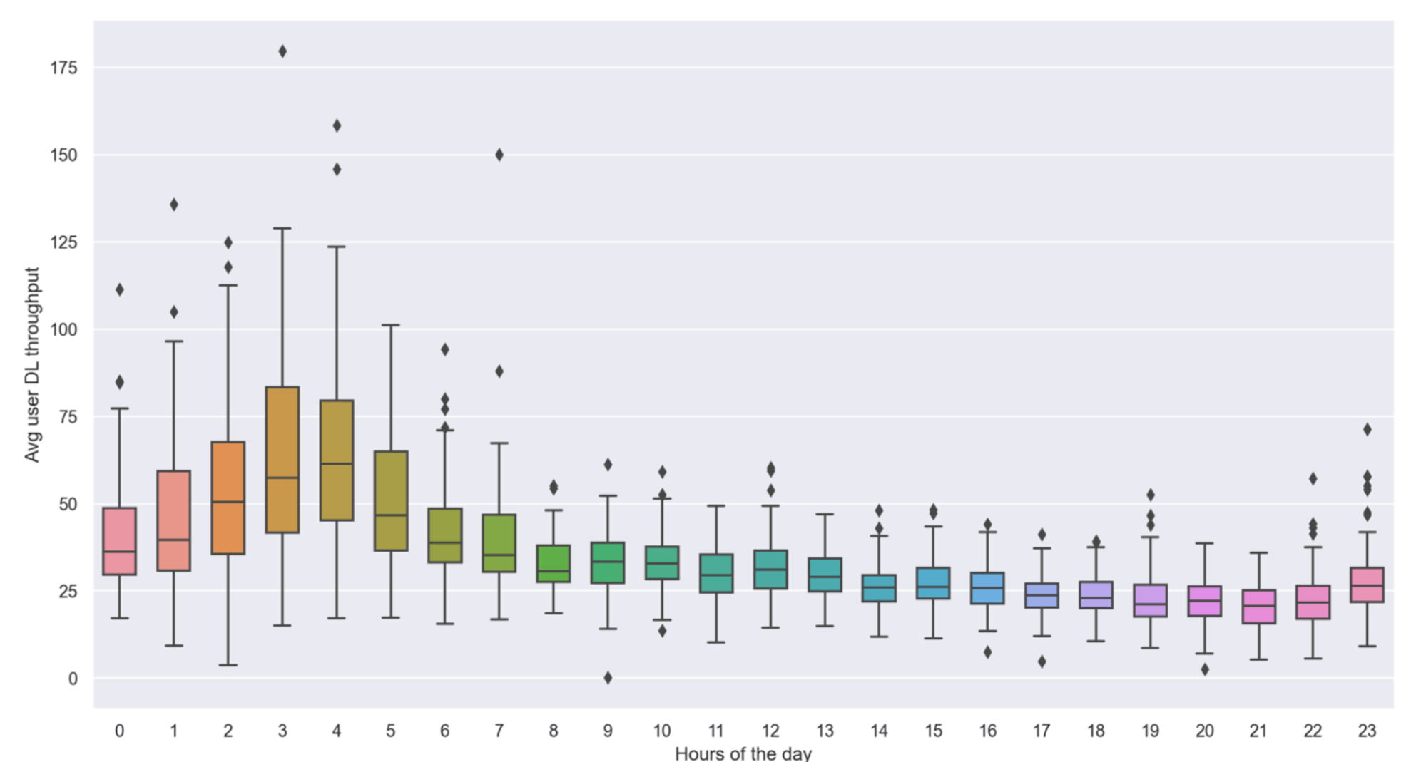Figure 2. Network traffic variation over 24 hour period

Step 2: time series decomposition

Our next step was to apply time series decomposition to the data. This technique breaks time series into their three primary components:

• Trend - representing the overall increase or decrease in a series over time
• Seasonality - representing periodic cycles in a series
• Noise - representing random variation in a series

Figure 3 shows the time series decomposition of the KPI from one of the cells under study.

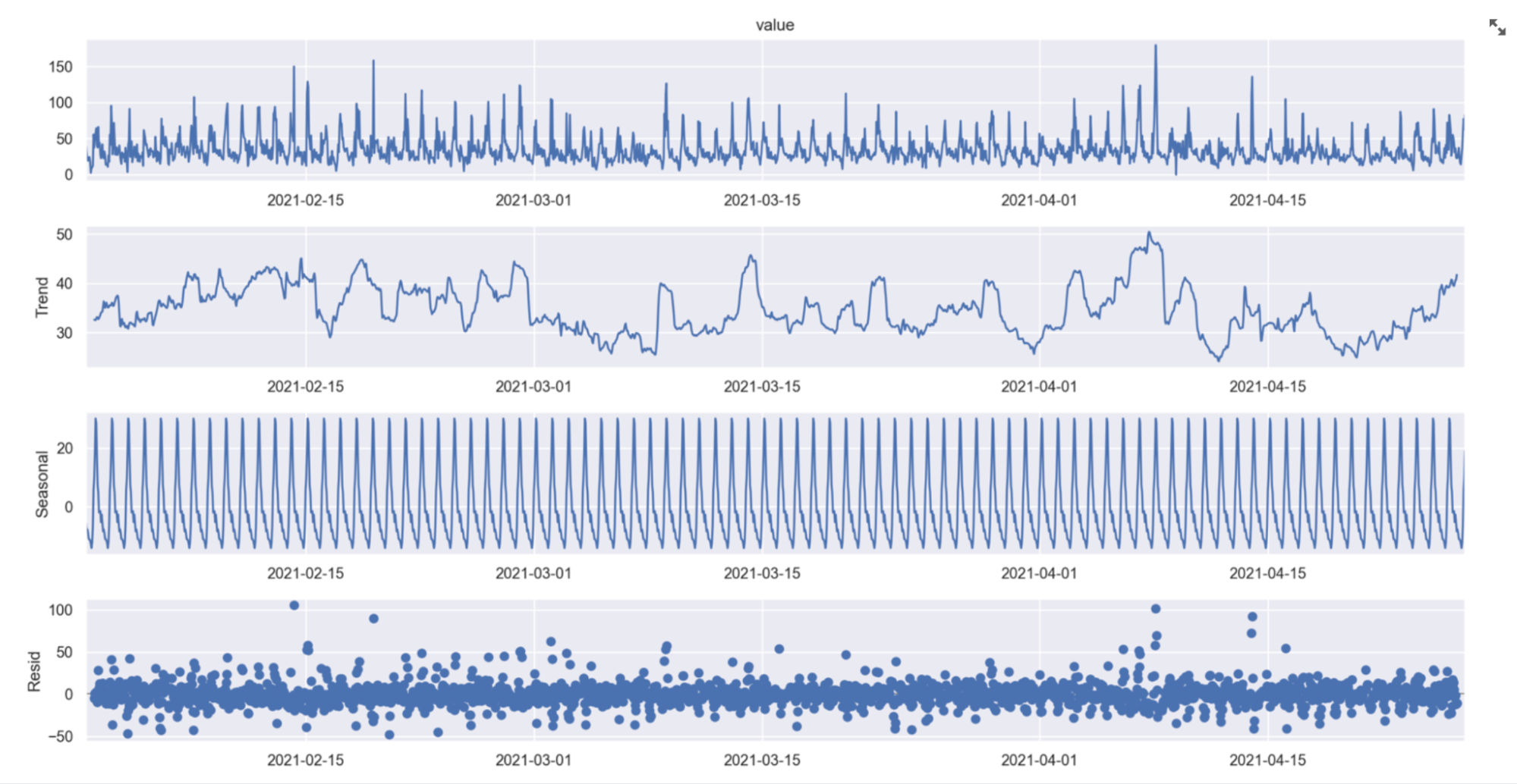Figure 3. Time series seasonal decomposition

Step 3: data preprocessing

We need a model that learns to focus on lower KPI values and not be distracted by higher ones so that it can better predict future dips. To achieve this, we transform the KPI by taking the minimum value across a 3-hour rolling window and using that transformed data to train our model.

Step 4: model selection

A combination of classical time series models, such as the Simple Moving Average (SMA) or Autoregressive Integrated Moving Average (ARIMA) are often used to forecast time series. These approaches, however, are suited for short term forecasts and capture only the linear dependencies present in the data. We were working with data that had missing values, a combination of linear and non-linear dependencies, and noise. Furthermore, at any given time, the value of the KPI (average downlink throughput) can be affected by a large number of factors. These factors (influencers) often do not behave as we might think they should; the interplay between linearity and nonlinearity is subtle and complex, so we needed a technique that could model this interplay.

Instead, we chose the Long Short-Term Memory (LSTM) technique, a popular time series modelling framework due to its ability to forecast for longer time horizons and automatic feature extraction abilities. Add to that its end-to-end modelling and automatic feature extraction capabilities that relieves developers of much of preprocessing and manual feature engineering work.

LSTMs have emerged as one of the most effective solutions for sequence prediction problems and can be found powering autocorrect and autocomplete features in applications as varied as iPhone autocorrect, and Google Docs auto-complete. They have the edge over conventional feed-forward neural networks and recurrent neural networks (RNN) in many ways because of their property of selectively remembering patterns for longer durations. It was for this reason that we chose the LSTM model for our RAN congestion problem.

Step 5: model training

Using hourly values over 3 months of historical KPI data from one cell to train the forecasting model to learn trends, seasonality and predict values for 7 days into the future, we compared the Mean Absolute Percentage Error (MAPE) performance of a variety of models (Prophet, LSTM, ARIMA, SARIMA). We trained the model on 80% of the data and kept 20% for testing to determine how accurate the predicted values were in relation to the actual values.

The best performing model was Long Short-Term Memory (LSTM), implemented using TensorFlow. LSTM uses the same architecture as RNN but is capable of dealing with more complex problems by keeping a constant flow of error throughout the backpropagation from one cell to another. It operates by learning a function that maps a sequence of inputs to a sequence of outputs.

Consider an example where we have to build a model to predict the next number in the following sequence [10, 20, 30, 40, 50, 60, 70, 80, 90]. Using LSTM, we can divide the sequence into multiple input/output patterns, where three time steps [10,20,30] are used as input and the following time step output [40]. Following this, [20,30,40] becomes the new input and the output we are trying to predict is [50].

The sequence of observations (the pattern which the values of the KPI follow) must be transformed into multiple examples from which the LSTM can learn so we had to frame the problem as a regression problem wherein we used a lookback of 6 hours. The training dataset for our neural network required sliding windows X (input) and Y (output) of desired lag (lookback of 6 hours), as well as a forecast horizon (7 days). Using these two windows, we trained an LSTM Network consisting of 3 stacked LSTM layers and 3 fully connected layers along with the final output layer (as shown in figure 4) by minimizing a loss function, in this case, mean squared error.

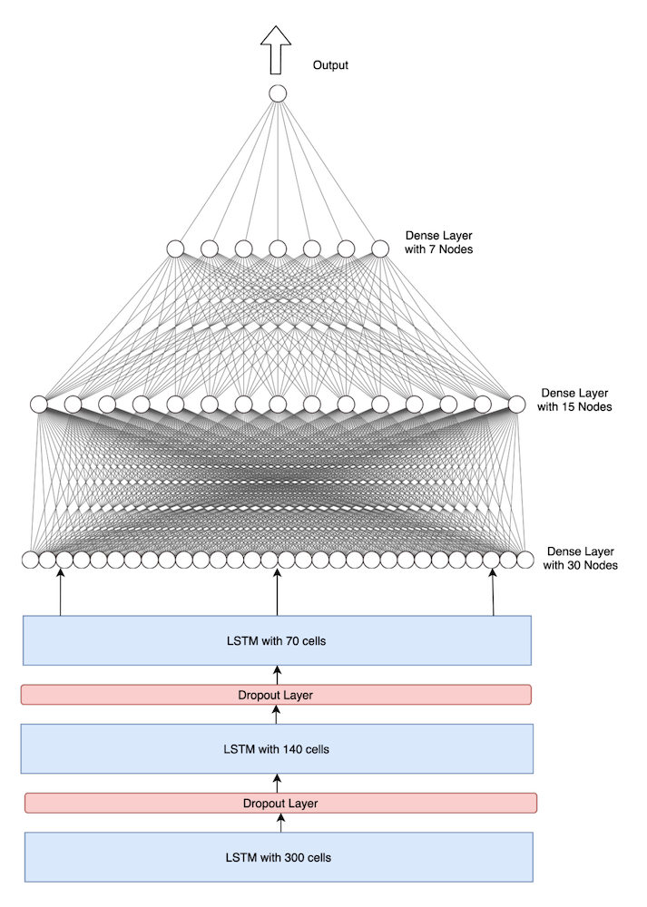Figure 4. LSTM model architecture

Step 6: further testing and initial results

During testing, we consistently achieved a MAPE of less than 10%. Figure 5 below shows the model performance compared to the actual observations.

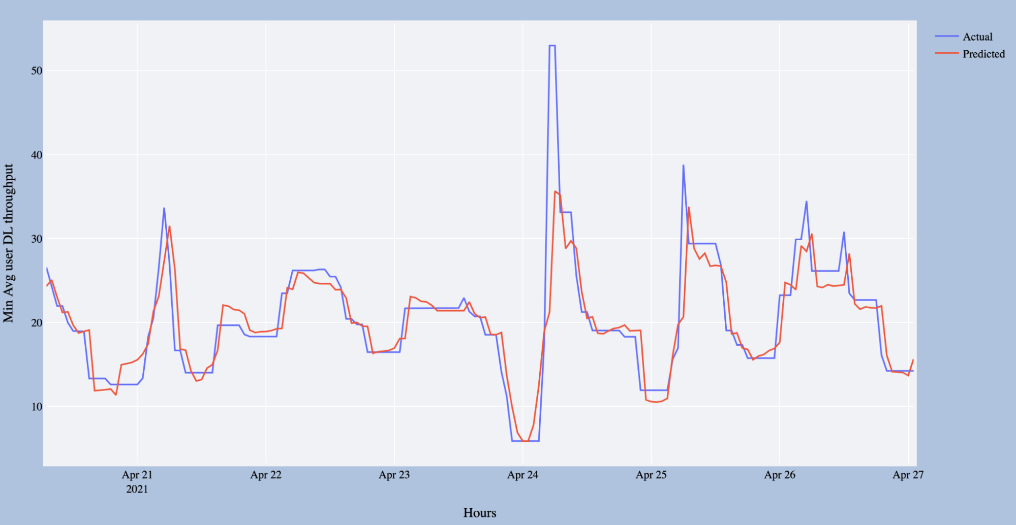Figure 5. seven day forecast

The model accurately predicts the minimum values of the KPI for all seven days, thus making it incredibly useful for not only predicting the congestion but predicting the services that would be impacted by the congestion.

Figure 6 below shows the services impacted when the KPI falls below the thresholds required to ensure service quality. As the model can predict up to seven days advance notice, operators have time to take steps to mitigate any impact.

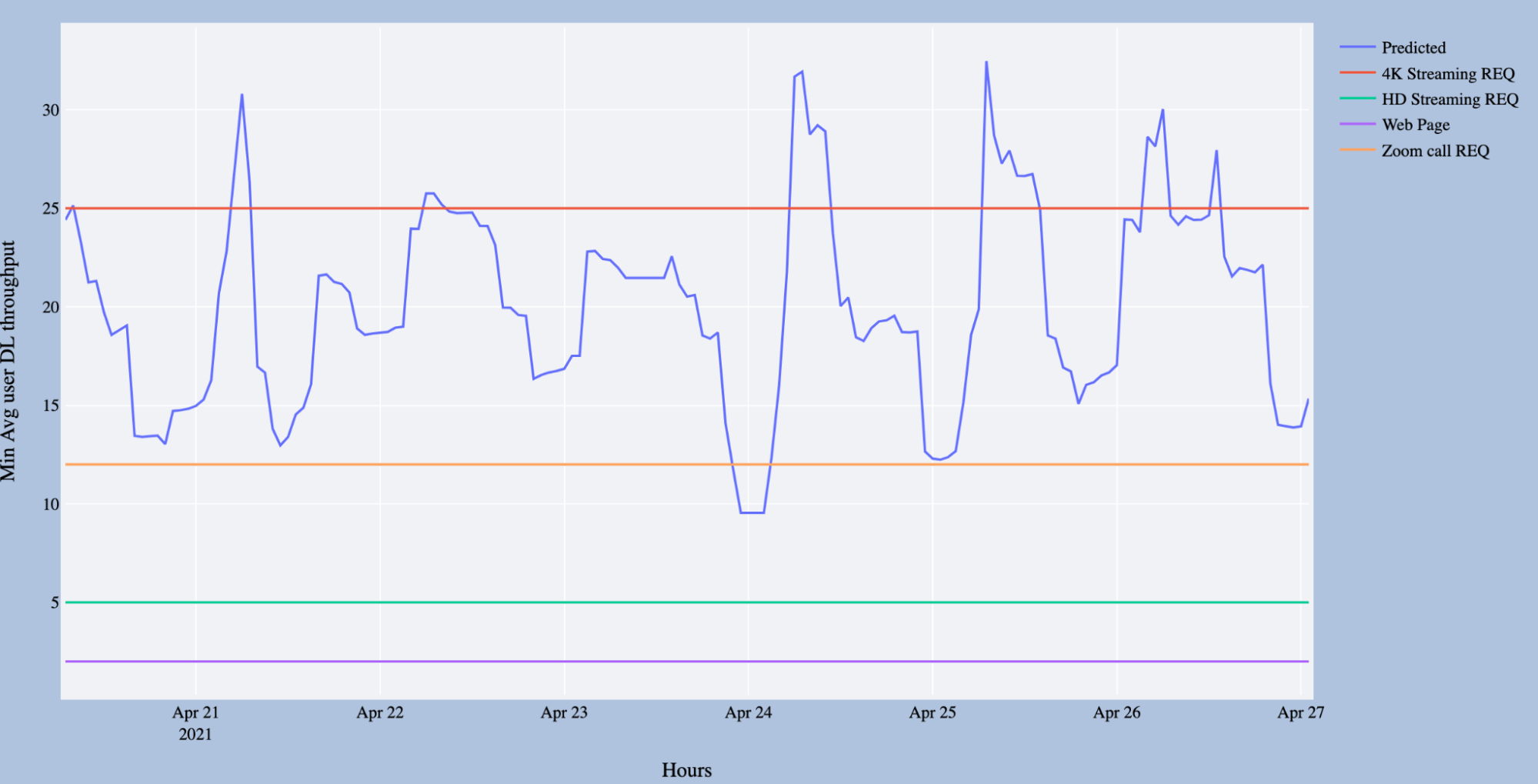Figure 6. KPI forecast with quality of service thresholds

Next steps

With our model developed, we now plan to integrate this functionality into VisiMetrix so that our customers can reap the benefits of forecasting on their production dashboards. We’re looking forward to seeing it in action in the wild on 2G, 3G, 4G, 5G networks.

If you’d like to learn out more about VisiMetrix, visit visimetrix.com